Statistical notes for clinical researchers: covariance and correlation

Hae-Young Kim

doi:10.5395/rde.2018.43.e4

Articles

Page Path: HOME > Restor Dent Endod > Volume 43(1); 2018 > Article

Open Lecture on Statistics Statistical notes for clinical researchers: covariance and correlation: Hae-Young Kim; Restor Dent Endod 2018;43(1):e4.
DOI: https://doi.org/10.5395/rde.2018.43.e4
Published online: January 5, 2018

Department of Health Policy and Management, College of Health Science, and Department of Public Health Science, Graduate School, Korea University, Seoul, Korea.

Correspondence to Hae-Young Kim, DDS, PhD. Department of Health Policy and Management, College of Health Science, and Department of Public Health Science, Graduate School, Korea University, 145 Anam-ro, Seongbuk-gu, Seoul 02841, Korea. Tel: +82-2-3290-5667, Fax: +82-2-940-2879, kimhaey@korea.ac.kr

This is an Open Access article distributed under the terms of the Creative Commons Attribution Non-Commercial License (https://creativecommons.org/licenses/by-nc/4.0/) which permits unrestricted non-commercial use, distribution, and reproduction in any medium, provided the original work is properly cited.

1,113 Views
8 Download
12 Crossref

prev next

Full Article

Download PDF

COVARIANCE
PEARSON CORRELATION COEFFICIENT
SPEARMAN'S RANK CORRELATION COEFFICIENT
REFERENCES
Appendix

Covariance and correlation are basic measures describing the relationship between two variables. They are a broad class of statistical tools which evaluate how two variables are related with dependence or association, especially for linear relationship. Difference between the two is that covariance is calculated under the original units of two variables, while correlation is obtained based on standardized scale resulting in a unit-less measure.

COVARIANCE

Covariance is defined as the expected value of variations of two variables from their expected values. More simply, covariance measures how much variables change together. The mean of each variable is used as reference and relative positions of observations compared to mean is important. Covariance is simply defined as the mean of multiplication of corresponding X and Y deviations from their mean,

$(X-X-)$

and

$(Y-Y-)$

. Covariance is expressed as following formula:

$CovarianceX,Y=∑(X-X-)(Y-Y-)n-1$

where n is the number of X and Y pairs.

Covariance mainly represents the direction of relationship of two variables. A positive sign of covariance value represents that two variables move to the same direction while a negative covariance value means that two variables move to opposite directions. Figure 1 shows a coordinate plane made by the line X and Y (dotted line) as well as

$X-$

= 5 and

$Y-$

= 6 (solid line). In the quadrant I, x value moves positively from its mean and so does y value. Therefore, the points in the quadrant I represent positive relationship between two variables because Y values get larger as X values get larger relatively to their mean. Similarly, the points in the quadrant III also represent positive relationship because Y values get smaller than its mean as X values get smaller. The sign of the multiplicative value of each deviation,

$X-X-Y-Y-$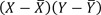

is positive in the quadrants I and III because the pair of deviations have the same sign that both are positive or negative. Contrary, the points in quadrants II and IV show negative relationship as one variable gets larger than its mean as the other gets smaller (Figure 1). In quadrants II and IV, the sign of the multiplicative value of each deviation is negative because the pair of deviations have different signs each other.

Figure 1

Illustration of relative positions of two variables in reference to their means.

Download Figure

A positive sign of covariance means that points in the quadrants I and III are predominant than those in the quadrants II and IV. A negative sign represents predominance of points in the quadrants II and IV. Therefore, positive and negative signs of covariance values can be interpreted as positive and negative relationships between 2 variables, respectively. If the covariance value is near zero, we may interpret there is no clear positive or negative relationship. The example data in Table 1 shows positive covariance value, 109.1, which means a positive, increasing relationship between X and Y.

Table 1

The calculation procedure of covariance and Pearson correlation coefficient

No	X	Y	X−X̄	Y−Ȳ	(X−X̄)²	(Y−Ȳ)²	(X−X̄)(Y−Ȳ)
1	73	90	0.55	7.65	0.30	58.52	4.21
2	52	74	−20.45	−8.35	418.20	69.72	170.76
3	68	91	−4.45	8.65	19.80	74.82	−38.49
4	47	62	−25.45	−20.35	647.70	414.12	517.91
5	60	63	−12.45	−19.35	155.00	374.42	240.91
6	71	78	−1.45	−4.35	2.10	18.92	6.31
7	67	60	−5.45	−22.35	29.70	499.52	121.81
8	80	89	7.55	6.65	57.00	44.22	50.21
9	86	82	13.55	−0.35	183.60	0.12	−4.74
10	91	105	18.55	22.65	344.10	513.02	420.16
11	67	76	−5.45	−6.35	29.70	40.32	34.61
12	73	82	0.55	−0.35	0.30	0.12	−0.19
13	71	93	−1.45	10.65	2.10	113.42	−15.44
14	57	73	−15.45	−9.35	238.70	87.42	144.46
15	86	82	13.55	−0.35	183.60	0.12	−4.74
16	76	88	3.55	5.65	12.60	31.92	20.06
17	91	97	18.55	14.65	344.10	214.62	271.76
18	69	80	−3.45	−2.35	11.90	5.52	8.11
19	87	87	14.55	4.65	211.70	21.62	67.66
20	77	95	4.55	12.65	20.70	160.02	57.56
	X̄ = 72.45	Ȳ = 82.35			∑ = 2,912.95	∑ = 2,742.55	∑ = 2,072.85

$CovarianceX,Y=∑X-X-Y-Y-n-1=2,072.8520-1=109.10,$

$SDX=∑X-X-2n-1=2,912.9520-1=12.38,SDY=∑Y-Y-2n-1=2,742.5520-1=12.01,$

$Pearson correlation coefficient (r)=Cov(x,y)SDX × SD(Y)=109.1012.38 × 12.01=0.73.$

Download Table

Then what can we say about the size of covariance values? Magnitude of the relationship? However, the problem is that the absolute value of covariance depends on the unit of variables. For example, if we change the unit of a variable from kilometer to meter unit, then the deviance from mean of 1 in kilometer units (km) is changed into 1,000 in meter units (m). The unit change makes huge difference in the value of covariance, even when the relationship of 2 variables is the same. Therefore, the size of covariance value cannot be interpretable as the magnitude of a relationship. Also, a covariance value has neither upper or lower bound nor any standard to determine the degree of relationship. There is a need of unit standardization procedure on covariance.

Table 1 shows the calculation procedure of covariance and Pearson correlation coefficient. Deviations of X and Y are multiplied, summed-up, and finally divided by n-1 to get covariance value. The Pearson correlation coefficient is obtained by dividing covariance value with standard deviations (SDs) of X and Y variables.

PEARSON CORRELATION COEFFICIENT

Correlation is the standardized form of covariance by dividing the covariance with SD of each variable under normal distribution assumption. Generally, we use ‘r’ as sample correlation coefficient and ‘ρ’ as population correlation coefficient. The Pearson correlation coefficient has following formula.

$Pearson Correlation coefficient (ρ or r)=Cov(x,y)SDX × SD(Y)$

The Pearson correlation coefficient is also the covariance of standardized form of X and Y variables. The correlation coefficient is unit-less, being independent of the scale of variables and the range is between −1 and +1. The interpretation of the Pearson correlation coefficient was provided by Cohen [1]. He proposed a small, medium, and large effect size of r as 0.1, 0.3, and 0.5, respectively, and explained that the medium effect size represents an effect likely to be visible to the naked eye of a careful observer. Also he subjectively set a small effect size to be noticeably smaller than medium but not so small as to be trivial and set a large effect size to be the same distance above the medium as small was below it [1]. His standard is generally accepted at the present.

Because the correlation coefficient reflects only the strength of linear relationship, we need a cautious investigation of scatterplot before calculating it. As shown in Figure 2, a correlation coefficient of 0.8 can be obtained from totally different relationships between two variables. Only Figure 2A shows correct linear relationship, while curved relationship (Figure 2B), distorting effect of an outlier (Figure 2C), and strong effect of an outlier on the unrelated relationship (Figure 2D) show some relations different from a linear one. We need to keep in mind that all these different shapes of relationships could result in the same correlation coefficient. We should check those possibilities using scatterplots.

Figure 2

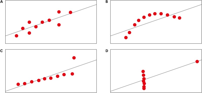
Four different relationship of two variables with the same correlation coefficient of around 0.8.

Download Figure

If the correlation coefficient is zero, there is also some caution needed in interpreting the meaning. We may expect no relationship such as Figure 3A, the shape of random scatter. However, U shape or reverse U shape relationship can show zero correlation coefficient (Figure 3B and 3C). An example of U shape relationship is the relationship between consumption of electricity and temperature. At very low temperature lots of electricity is consumed for warming and the need is gradually decreased with the increase of temperature. However, if temperature rises further we need more electricity for air conditioning. An example of reverse U shape is the relationship between stress and work performance. Performance may be improved if there is some stress, but too much stress can cause burn-out of the person which decreases performance. Therefore, it is always a good idea to examine the relationship between variables with a scatterplot.

Figure 3

Typical types of zero correlation: (A) random scatter — true no association, (B) U shape, and (C) reverse U shape.

Download Figure

SPEARMAN'S RANK CORRELATION COEFFICIENT

Spearman's rank correlation coefficient is the non-parametric version of the Pearson correlation coefficient calculated using rank values of two variables. It is expressed as following formula.

$Spearman correlation coefficient ρ or rs=1-6∑d2nn2-1 ,$

where d = Rank(Y) − Rank(X) and n = sample size.

While the Pearson correlation assesses linear relationships, Spearman correlation assesses monotonic relationship that two variables are related but not necessarily linear. Let’s consider the relationship between 99 p values ranges from 0.01 to 0.99 by 0.01-unit increase and corresponding log odds values,

$lnp1-p$

. As seen Figure 4, Spearman correlation coefficient is 1 when y values always increase as x values increase, while Pearson correlation coefficient counts only linearity with coefficient of 0.97. Spearman rank correlation coefficient can be applied on continuous variables with influential outliers which are located far away from most observations. In such cases, it is not appropriate to apply Pearson. Also, it can be applied to assess relationships between ordered categorical values. The range of Spearman correlation coefficient is from −1 to +1, which represent perfect negative and positive relationships, respectively.

Figure 4

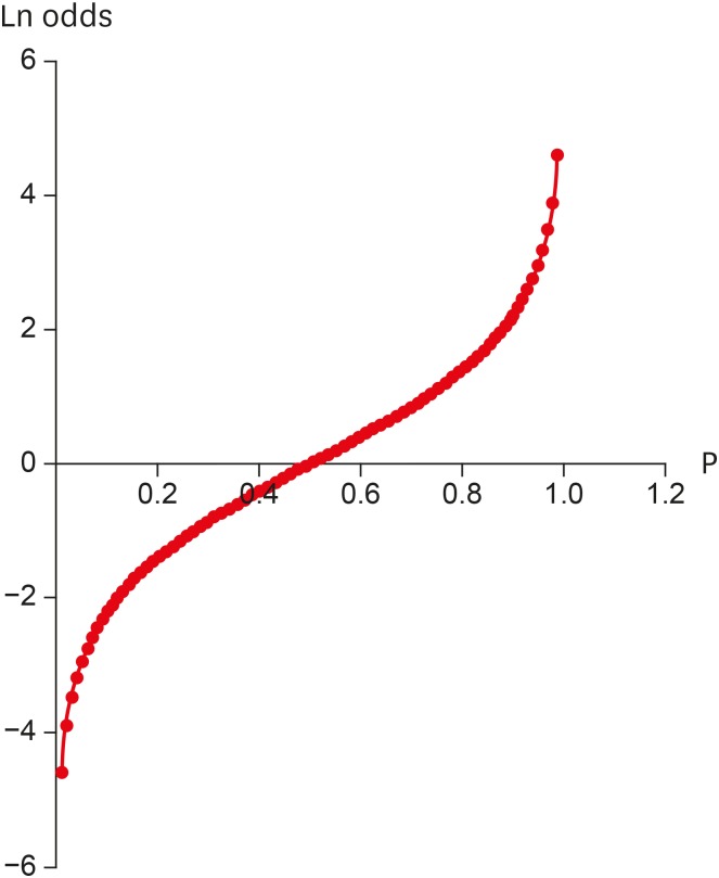
A curved relationship of ‘p’ and ‘ln odds’. (Pearson correlation = 0.97 vs. Spearman's rank correlation = 1).

Download Figure

Table 2 shows the calculation procedure of the Spearman rank correlation. Difference of rank of two variables is used in calculating rank correlation coefficient.

Table 2

The calculation procedure of the Spearman's rank correlation

No	X	Y	Rank(X)	Rank(Y)	d^*	d²
1	73	90	11.5	15	3.5	12.25
2	52	74	2	5	3	9
3	68	91	7	16	9	81
4	47	62	1	2	1	1
5	60	63	4	3	−1	1
6	71	78	9.5	7	−2.5	6.25
7	67	60	5.5	1	−4.5	20.25
8	80	89	15	14	−1	1
9	86	82	16.5	10	−6.5	42.25
10	91	105	19.5	20	0.5	0.25
11	67	76	5.5	6	0.5	0.25
12	73	82	11.5	10	−1.5	2.25
13	71	93	9.5	17	7.5	56.25
14	57	73	3	4	1	1
15	86	82	16.5	10	−6.5	42.25
16	76	88	13	13	0	0
17	91	97	19.5	19	−0.5	0.25
18	69	80	8	8	0	0
19	87	87	18	12	−6	36
20	77	95	14	18	4	16
						∑ = 328.5

$Spearman's correlation coefficient rs=1-6∑d2nn2-1=1-6 × 328.520202-1=1-0.25=0.75.$

^*d = Rank(Y) − Rank(X).

Download Table

REFERENCES

1. Cohen J. A power primer. Psychol Bull 1992;112:155-159.Article PubMed

Appendix 1

Tables & Figures

Figure 1

Illustration of relative positions of two variables in reference to their means.

Download Figure

Table 1

The calculation procedure of covariance and Pearson correlation coefficient

No	X	Y	X−X̄	Y−Ȳ	(X−X̄)²	(Y−Ȳ)²	(X−X̄)(Y−Ȳ)
1	73	90	0.55	7.65	0.30	58.52	4.21
2	52	74	−20.45	−8.35	418.20	69.72	170.76
3	68	91	−4.45	8.65	19.80	74.82	−38.49
4	47	62	−25.45	−20.35	647.70	414.12	517.91
5	60	63	−12.45	−19.35	155.00	374.42	240.91
6	71	78	−1.45	−4.35	2.10	18.92	6.31
7	67	60	−5.45	−22.35	29.70	499.52	121.81
8	80	89	7.55	6.65	57.00	44.22	50.21
9	86	82	13.55	−0.35	183.60	0.12	−4.74
10	91	105	18.55	22.65	344.10	513.02	420.16
11	67	76	−5.45	−6.35	29.70	40.32	34.61
12	73	82	0.55	−0.35	0.30	0.12	−0.19
13	71	93	−1.45	10.65	2.10	113.42	−15.44
14	57	73	−15.45	−9.35	238.70	87.42	144.46
15	86	82	13.55	−0.35	183.60	0.12	−4.74
16	76	88	3.55	5.65	12.60	31.92	20.06
17	91	97	18.55	14.65	344.10	214.62	271.76
18	69	80	−3.45	−2.35	11.90	5.52	8.11
19	87	87	14.55	4.65	211.70	21.62	67.66
20	77	95	4.55	12.65	20.70	160.02	57.56
	X̄ = 72.45	Ȳ = 82.35			∑ = 2,912.95	∑ = 2,742.55	∑ = 2,072.85

$CovarianceX,Y=∑X-X-Y-Y-n-1=2,072.8520-1=109.10,$

$SDX=∑X-X-2n-1=2,912.9520-1=12.38,SDY=∑Y-Y-2n-1=2,742.5520-1=12.01,$

$Pearson correlation coefficient (r)=Cov(x,y)SDX × SD(Y)=109.1012.38 × 12.01=0.73.$

Download Table

Figure 2

Four different relationship of two variables with the same correlation coefficient of around 0.8.

Download Figure

Figure 3

Typical types of zero correlation: (A) random scatter — true no association, (B) U shape, and (C) reverse U shape.

Download Figure

Figure 4

A curved relationship of ‘p’ and ‘ln odds’. (Pearson correlation = 0.97 vs. Spearman's rank correlation = 1).

Download Figure

Table 2

The calculation procedure of the Spearman's rank correlation

No	X	Y	Rank(X)	Rank(Y)	d^*	d²
1	73	90	11.5	15	3.5	12.25
2	52	74	2	5	3	9
3	68	91	7	16	9	81
4	47	62	1	2	1	1
5	60	63	4	3	−1	1
6	71	78	9.5	7	−2.5	6.25
7	67	60	5.5	1	−4.5	20.25
8	80	89	15	14	−1	1
9	86	82	16.5	10	−6.5	42.25
10	91	105	19.5	20	0.5	0.25
11	67	76	5.5	6	0.5	0.25
12	73	82	11.5	10	−1.5	2.25
13	71	93	9.5	17	7.5	56.25
14	57	73	3	4	1	1
15	86	82	16.5	10	−6.5	42.25
16	76	88	13	13	0	0
17	91	97	19.5	19	−0.5	0.25
18	69	80	8	8	0	0
19	87	87	18	12	−6	36
20	77	95	14	18	4	16
						∑ = 328.5

$Spearman's correlation coefficient rs=1-6∑d2nn2-1=1-6 × 328.520202-1=1-0.25=0.75.$

^*d = Rank(Y) − Rank(X).

Download Table

REFERENCES

1. Cohen J. A power primer. Psychol Bull 1992;112:155-159.Article PubMed

Citations

Citations to this article as recorded by

Occupational Lead Exposure Among Civilian Indoor Shooting Range Workers in Korea: A Report of Blood Lead Levels and Airborne Lead
Sungjin Park, Jaeyoung Park, Bumjoon Lee, Yi-Ryoung Lee, Jiho Kim, Younmo Cho, Hyeongyeong Choi, Kyeongyeon Kim
Journal of Korean Medical Science.2025;[Epub] CrossRef
Improving the forecast accuracy of wind power by leveraging multiple hierarchical structure
Lucas English, Mahdi Abolghasemi
Sustainable Energy, Grids and Networks.2024; 40: 101517. CrossRef
Simplified Methods for Modelling Dependent Parameters in Health Economic Evaluations: A Tutorial
Xuanqian Xie, Alexis K. Schaink, Sichen Liu, Myra Wang, Juan David Rios, Andrei Volodin
Applied Health Economics and Health Policy.2024; 22(3): 331. CrossRef
Numerical modeling of ocean currents and suspended sediment distribution in Benoa Bay, Bali
Siti Sulistiana, I Wayan Nurjaya, Mochamad Tri Hartanto, H.M. Manik, N.P. Zamani, J. Lumban Gaol, A.S. Atmadipoera, O. Meng Chuan, T. Osawa
BIO Web of Conferences.2024; 106: 03005. CrossRef
The effectiveness of the TRACE online nutrition intervention in improving dietary intake, sleep quality and physical activity levels for Australian adults with food addiction: a randomised controlled trial
Mark Leary, Janelle A. Skinner, Kirrilly M. Pursey, Antonio Verdejo‐Garcia, Rebecca Collins, Clare Collins, Phillipa Hay, Tracy L. Burrows
Journal of Human Nutrition and Dietetics.2024; 37(4): 978. CrossRef
Influence of the radius of Monson’s sphere and excursive occlusal contacts on masticatory function of dentate subjects
Dominique Ellen Carneiro, Luiz Ricardo Marafigo Zander, Carolina Ruppel, Giancarlo De La Torre Canales, Rubén Auccaise-Estrada, Alfonso Sánchez-Ayala
Archives of Oral Biology.2024; 159: 105879. CrossRef
Analytical Performance Specifications for Input Variables: Investigation of the Model of End-Stage Liver Disease
Eline S Andersen, Richard Röttger, Claus L Brasen, Ivan Brandslund
Clinical Chemistry.2024; 70(4): 653. CrossRef
A prototype variable corresponding to the proportion of ischemia for the comparison between robotic and open partial nephrectomy: a meta-analysis accompanied by sensitivity analysis
Sotirios Artsitas, Dimitrios Artsitas, Irene Koronaki, Konstantinos G. Toutouzas, George C. Zografos
Beni-Suef University Journal of Basic and Applied Sciences.2023;[Epub] CrossRef
Cephalometric determinants of facial attractiveness: A quadratic correlation study
Joana Godinho, Diana Fernandes, Patrícia Pires, Luis Jardim
American Journal of Orthodontics and Dentofacial Orthopedics.2023; 163(3): 398. CrossRef
Sympathovagal Balance Is a Strong Predictor of Post High-Volume Endurance Exercise Cardiac Arrhythmia
Daniel W. T. Wundersitz, Bradley J. Wright, Brett A. Gordon, Stephanie Pompei, Carl J. Lavie, Voltaire Nadurata, Kimberly Nolan, Michael I. C. Kingsley
Frontiers in Physiology.2022;[Epub] CrossRef
Performance investigation of the natural draft wet cooling tower at different wet-bulb temperatures
Gaurav Raj, Prakash Chandra, Piyush Kumar Pathak
International Journal of Ambient Energy.2022; 43(1): 5864. CrossRef
Statistical notes for clinical researchers: simple linear regression 1 – basic concepts
Hae-Young Kim
Restorative Dentistry & Endodontics.2018;[Epub] CrossRef

CanvasJS.com

ePub Link

Cite

CITE: export Copy Download Format; Close

Download Citation

Download a citation file in RIS format that can be imported by all major citation management software, including EndNote, ProCite, RefWorks, and Reference Manager.

Format:

RIS — For EndNote, ProCite, RefWorks, and most other reference management software
BibTeX — For JabRef, BibDesk, and other BibTeX-specific software

Include:

Citation for the content below
Citation and abstract for the content below

Statistical notes for clinical researchers: covariance and correlation

Restor Dent Endod. 2018;43(1):e4 Published online January 5, 2018

DOI: https://doi.org/10.5395/rde.2018.43.e4

XML Download

Figure

Statistical notes for clinical researchers: covariance and correlation

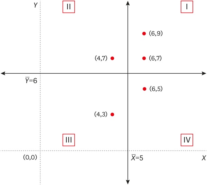
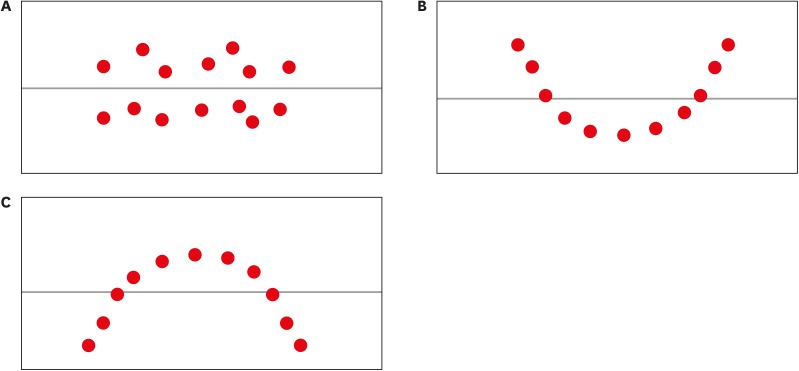
Figure 1 Illustration of relative positions of two variables in reference to their means.

Figure 2 Four different relationship of two variables with the same correlation coefficient of around 0.8.

Figure 3 Typical types of zero correlation: (A) random scatter — true no association, (B) U shape, and (C) reverse U shape.

Figure 4 A curved relationship of ‘p’ and ‘ln odds’. (Pearson correlation = 0.97 vs. Spearman's rank correlation = 1).

Figure 1

Figure 2

Figure 3

Figure 4

Statistical notes for clinical researchers: covariance and correlation

Table 1

The calculation procedure of covariance and Pearson correlation coefficient

No	X	Y	X−X̄	Y−Ȳ	(X−X̄)²	(Y−Ȳ)²	(X−X̄)(Y−Ȳ)
1	73	90	0.55	7.65	0.30	58.52	4.21
2	52	74	−20.45	−8.35	418.20	69.72	170.76
3	68	91	−4.45	8.65	19.80	74.82	−38.49
4	47	62	−25.45	−20.35	647.70	414.12	517.91
5	60	63	−12.45	−19.35	155.00	374.42	240.91
6	71	78	−1.45	−4.35	2.10	18.92	6.31
7	67	60	−5.45	−22.35	29.70	499.52	121.81
8	80	89	7.55	6.65	57.00	44.22	50.21
9	86	82	13.55	−0.35	183.60	0.12	−4.74
10	91	105	18.55	22.65	344.10	513.02	420.16
11	67	76	−5.45	−6.35	29.70	40.32	34.61
12	73	82	0.55	−0.35	0.30	0.12	−0.19
13	71	93	−1.45	10.65	2.10	113.42	−15.44
14	57	73	−15.45	−9.35	238.70	87.42	144.46
15	86	82	13.55	−0.35	183.60	0.12	−4.74
16	76	88	3.55	5.65	12.60	31.92	20.06
17	91	97	18.55	14.65	344.10	214.62	271.76
18	69	80	−3.45	−2.35	11.90	5.52	8.11
19	87	87	14.55	4.65	211.70	21.62	67.66
20	77	95	4.55	12.65	20.70	160.02	57.56
	X̄ = 72.45	Ȳ = 82.35			∑ = 2,912.95	∑ = 2,742.55	∑ = 2,072.85

$Covariance (X, Y) = \frac{\sum (X - \bar{X}) (Y - \bar{Y})}{n - 1} = \frac{2,072.85}{20 - 1} = 109.10,$

$\begin{matrix} S D (X) = \sqrt{\frac{\sum {(X - \bar{X})}^{2}}{n - 1}} = \sqrt{\frac{2,912.95}{20 - 1}} = 12.38, & S D (Y) = \sqrt{\frac{\sum {(Y - \bar{Y})}^{2}}{n - 1}} = \sqrt{\frac{2,742.55}{20 - 1}} = 12.01, \end{matrix}$

$Pearson correlation coefficient (r) = \frac{C o v (x, y)}{S D (X) \times S D (Y)} = \frac{109.10}{12.38 \times 12.01} = 0.73 .$

Table 2

The calculation procedure of the Spearman's rank correlation

No	X	Y	Rank(X)	Rank(Y)	d^*	d²
1	73	90	11.5	15	3.5	12.25
2	52	74	2	5	3	9
3	68	91	7	16	9	81
4	47	62	1	2	1	1
5	60	63	4	3	−1	1
6	71	78	9.5	7	−2.5	6.25
7	67	60	5.5	1	−4.5	20.25
8	80	89	15	14	−1	1
9	86	82	16.5	10	−6.5	42.25
10	91	105	19.5	20	0.5	0.25
11	67	76	5.5	6	0.5	0.25
12	73	82	11.5	10	−1.5	2.25
13	71	93	9.5	17	7.5	56.25
14	57	73	3	4	1	1
15	86	82	16.5	10	−6.5	42.25
16	76	88	13	13	0	0
17	91	97	19.5	19	−0.5	0.25
18	69	80	8	8	0	0
19	87	87	18	12	−6	36
20	77	95	14	18	4	16
						∑ = 328.5

$Spearman's correlation coefficient (r_{s}) = 1 - \frac{6 \sum d^{2}}{n (n^{2} - 1)} = 1 - \frac{6 \times 328.5}{20 (20^{2} - 1)} = 1 - 0.25 = 0.75 .$

^*d = Rank(Y) − Rank(X).

Table 1 The calculation procedure of covariance and Pearson correlation coefficient

$CovarianceX,Y=∑X-X-Y-Y-n-1=2,072.8520-1=109.10,$

$SDX=∑X-X-2n-1=2,912.9520-1=12.38,SDY=∑Y-Y-2n-1=2,742.5520-1=12.01,$

$Pearson correlation coefficient (r)=Cov(x,y)SDX × SD(Y)=109.1012.38 × 12.01=0.73.$

Table 2 The calculation procedure of the Spearman's rank correlation

$Spearman's correlation coefficient rs=1-6∑d2nn2-1=1-6 × 328.520202-1=1-0.25=0.75.$

^*d = Rank(Y) − Rank(X).

Articles

COVARIANCE

The calculation procedure of covariance and Pearson correlation coefficient

PEARSON CORRELATION COEFFICIENT

SPEARMAN'S RANK CORRELATION COEFFICIENT

The calculation procedure of the Spearman's rank correlation

REFERENCES

Appendix

Procedure of covariance and correlation using IBM SPSS

Tables & Figures

The calculation procedure of covariance and Pearson correlation coefficient

The calculation procedure of the Spearman's rank correlation

REFERENCES

Citations

Figure 1

Figure 2

Figure 3

Figure 4

The calculation procedure of covariance and Pearson correlation coefficient

The calculation procedure of the Spearman's rank correlation

Table 1

Table 2