Statistical notes for clinical researchers: analysis of covariance (ANCOVA)

Article information

Restor Dent Endod. 2018;43.e43

Publication date (electronic) : 2018 October 22

doi : https://doi.org/10.5395/rde.2018.43.e43

Hae-Young Kim

Department of Health Policy and Management, College of Health Science, and Department of Public Health Science, Graduate School, Korea University, Seoul, Korea.

Correspondence to Hae-Young Kim, DDS, PhD. Professor, Department of Health Policy and Management, Korea University College of Health Science, and Department of Public Health Science, Korea University Graduate School, 145 Anam-ro, Seongbuk-gu, Seoul 02841, Korea. kimhaey@korea.ac.kr

RAISING A QUESTION ON IGNORING COVARIATES

An example data is composed of 3 variables, treatment effect, treatment methods (Tx; 2 groups), and age in Table 1. Our interest is on comparison of treatment effects by 2 Tx, experimental and control groups. We may consider independent t-test, ignoring age variable. Distribution of treatment effects of 2 groups is depicted in Figure 1A. We could obtain the p value, 0.048, by applying independent student's t-test comparing treatment groups and conclude the treatment effect of treatment group is superior to that of control group.

Table 1

Data of treatment groups, treatment effect (Effect), and age (Age)

Figure 1

Scatter plot of the example data in Table 1. (A) Distribution of treatment effects of 2 groups; (B) Scatter plot of treatment effects and age by treatment groups.

Now let's look into the relationship between treatment effect and age. We can notice a trend that higher age is related to higher treatment effect in Figure 1B. The positive correlation between effect and age is quantitatively measured by a Pearson correlation coefficient, 0.805 (p < 0.001). The positive correlation is further analyzed by regression analysis. We get regression equations for pooled sample of both groups as well as for each group as following:

Meanwhile, the mean age of subjects in the experimental group is 44.83 years, which is higher than that of the control group, 43.58 years. We may be suspicious that the difference of effect between two groups is partly attributed to the age difference between two groups, because age is positively correlated with treatment effect. How can we resolve this issue? There is a clear need to consider the covariate, age, into the model to control its possible influence.

ANCOVA MODEL: COMPARING MEANS CONSIDERING COVARIATES

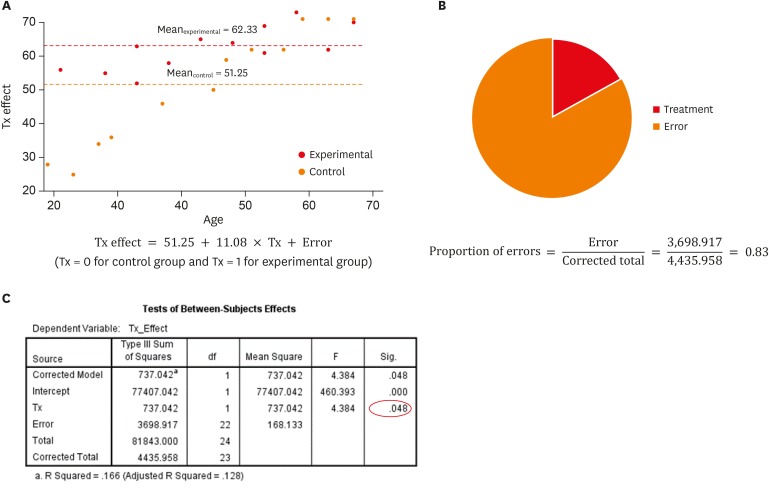
To compare 2 means, we can apply ANOVA as well, which is applicable in comparing 2 or more group means. The result shows significant difference between two groups (p = 0.048), which is exactly the same with that from the independent t-test in Figure 2C. Still, the possible covariate, age, is ignored. The model including 2 groups explains the variation of effect as much as corrected model sum of squares of 737.042 among total sum of squares of 4,435.958 in Figure 2C. Figure 2B displays the proportion of errors as 0.83, which is proportion of Error sum of squares of 3,698.917 among total sum of squares of 4,435.958. The proportion of errors represents the portion of variation that the model cannot explain. Also, we find the proportion of explained variance, R-squared, is 0.166, which represents that only 16.6% of variance in the response variable is explained by this model.

Figure 2

An analysis of variance (ANOVA) model considering 2 treatment methods (Tx). (A) Depiction of data and model; (B) Proportion of errors; (C) ANOVA table.

The ANOVA model can be performed using GLM procedure. The result is expressed as a GLM equation in Figure 2A, as:

where Tx = 0 for control group and Tx = 1 for experimental group.

We can obtain the mean effects of experimental and control groups as 62.33 (= 51.25 + 11.08) and 51.25, exactly the same as which appears above.

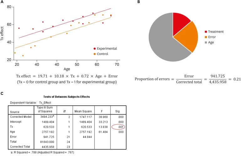
To solve the question whether different age levels influence the degree of group difference in treatment effect level, we include age into the model. We insert the covariate, age, into the previous ANOVA model, constructing an ANCOVA model. The result is shown in Figure 3. The resulting ANCOVA equation is:

Figure 3

An analysis of covariance (ANCOVA) model considering 2 treatment methods (Tx) and age as main effects. (A) Depiction of data and model; (B) Proportion of errors; (C) analysis of variance (ANOVA) table.

where Tx = 0 for control group and Tx = 1 for experimental group.

The difference of effect between 2 groups has changed slightly from 11.08 in Equation 4 to 10.18 in Equation 5. The size of intercept has reduced greatly by around 31 because it has been adjusted by age. One unit increase of age is related to an increase of 0.72 unit in treatment effect. The proportion of errors has decreased greatly from 0.83 to 0.21 in Figure 3B. The reason is because age explained a big portion of variability in the response variable (gray colored segment).

As appeared in Figure 3C, the proportion explained by the ANCOVA model has improved up to 78.8%, mainly due to the contribution of age variable. The p values of Tx and age are 0.01 and < 0.001, respectively, which represent a highly significant result. The inclusion of covariate which is highly correlated with response can remove a considerable portion of errors, reducing the proportion of errors. In contrast, the explanation ability and significance of factors increase in the ANCOVA model.

It is noticeable that the slope of age is the same as 0.72 for both treatment groups in Figure 3A, which is restricted by the assumption of the ANCOVA model. The slope is similar to that of pooled sample, 0.74 as appeared in Equation 1. However, the slopes of 2 groups may actually be different because the slopes of 2 groups seem substantially different from one another, 0.33 in Equation 2 and 1.03 in Equation 3.

ANCOVA MODEL WITH INTERACTION

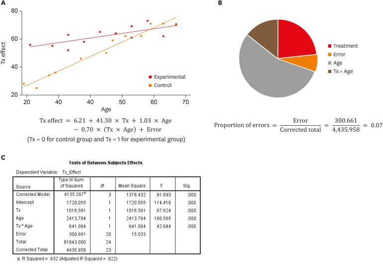
An ANCOVA model with interaction term is often called ‘a moderated regression,’ specifically [1]. Now we consider including an interaction term between group and age into the previous ANCOVA model, to assess if there is a significant difference in slopes of 2 groups. In Figure 3C, we find that the interaction term, Tx × Age, is statistically significant (p < 0.001), which supports the need of interaction term. By applying the model, the proportion of errors has decreased dramatically to 7%, as a considerable portion of variance is explained by the interaction term (Figure 4B). Also, 93.2% of total variance is explained by the model (R-squared = 0.932, Figure 4C).

Figure 4

Information on a model considering 2 treatment methods (Tx), age, and their interaction effect (Tx × Age). (A) Depiction of data and model; (B) Proportion of errors; (C) analysis of variance (ANOVA) table.

The construction of ANCOVA model with interaction results in the model as follows:

where Tx = 0 for control group and Tx = 1 for experimental group.

Immediately, Equation 6 can create two separate models for both control and experimental groups. The resulting Equation 7 and Equation 8 is exactly the same with the results obtained by simple regression, Equation 2 and Equation 3, respectively.

Article information Continued