Statistical notes for clinical researchers: covariance and correlation
Article information
Covariance and correlation are basic measures describing the relationship between two variables. They are a broad class of statistical tools which evaluate how two variables are related with dependence or association, especially for linear relationship. Difference between the two is that covariance is calculated under the original units of two variables, while correlation is obtained based on standardized scale resulting in a unit-less measure.
COVARIANCE
Covariance is defined as the expected value of variations of two variables from their expected values. More simply, covariance measures how much variables change together. The mean of each variable is used as reference and relative positions of observations compared to mean is important. Covariance is simply defined as the mean of multiplication of corresponding X and Y deviations from their mean,  and
and  . Covariance is expressed as following formula:

where n is the number of X and Y pairs.
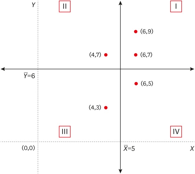
Covariance mainly represents the direction of relationship of two variables. A positive sign of covariance value represents that two variables move to the same direction while a negative covariance value means that two variables move to opposite directions. Figure 1 shows a coordinate plane made by the line X and Y (dotted line) as well as  = 5 and
  = 6 (solid line). In the quadrant I, x value moves positively from its mean and so does y value. Therefore, the points in the quadrant I represent positive relationship between two variables because Y values get larger as X values get larger relatively to their mean. Similarly, the points in the quadrant III also represent positive relationship because Y values get smaller than its mean as X values get smaller. The sign of the multiplicative value of each deviation,
  is positive in the quadrants I and III because the pair of deviations have the same sign that both are positive or negative. Contrary, the points in quadrants II and IV show negative relationship as one variable gets larger than its mean as the other gets smaller (Figure 1). In quadrants II and IV, the sign of the multiplicative value of each deviation is negative because the pair of deviations have different signs each other.
A positive sign of covariance means that points in the quadrants I and III are predominant than those in the quadrants II and IV. A negative sign represents predominance of points in the quadrants II and IV. Therefore, positive and negative signs of covariance values can be interpreted as positive and negative relationships between 2 variables, respectively. If the covariance value is near zero, we may interpret there is no clear positive or negative relationship. The example data in Table 1 shows positive covariance value, 109.1, which means a positive, increasing relationship between X and Y.
Then what can we say about the size of covariance values? Magnitude of the relationship? However, the problem is that the absolute value of covariance depends on the unit of variables. For example, if we change the unit of a variable from kilometer to meter unit, then the deviance from mean of 1 in kilometer units (km) is changed into 1,000 in meter units (m). The unit change makes huge difference in the value of covariance, even when the relationship of 2 variables is the same. Therefore, the size of covariance value cannot be interpretable as the magnitude of a relationship. Also, a covariance value has neither upper or lower bound nor any standard to determine the degree of relationship. There is a need of unit standardization procedure on covariance.
Table 1 shows the calculation procedure of covariance and Pearson correlation coefficient. Deviations of X and Y are multiplied, summed-up, and finally divided by n-1 to get covariance value. The Pearson correlation coefficient is obtained by dividing covariance value with standard deviations (SDs) of X and Y variables.
PEARSON CORRELATION COEFFICIENT
Correlation is the standardized form of covariance by dividing the covariance with SD of each variable under normal distribution assumption. Generally, we use ‘r’ as sample correlation coefficient and ‘ρ’ as population correlation coefficient. The Pearson correlation coefficient has following formula.

The Pearson correlation coefficient is also the covariance of standardized form of X and Y variables. The correlation coefficient is unit-less, being independent of the scale of variables and the range is between −1 and +1. The interpretation of the Pearson correlation coefficient was provided by Cohen [1]. He proposed a small, medium, and large effect size of r as 0.1, 0.3, and 0.5, respectively, and explained that the medium effect size represents an effect likely to be visible to the naked eye of a careful observer. Also he subjectively set a small effect size to be noticeably smaller than medium but not so small as to be trivial and set a large effect size to be the same distance above the medium as small was below it [1]. His standard is generally accepted at the present.
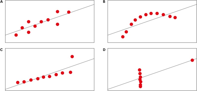
Because the correlation coefficient reflects only the strength of linear relationship, we need a cautious investigation of scatterplot before calculating it. As shown in Figure 2, a correlation coefficient of 0.8 can be obtained from totally different relationships between two variables. Only Figure 2A shows correct linear relationship, while curved relationship (Figure 2B), distorting effect of an outlier (Figure 2C), and strong effect of an outlier on the unrelated relationship (Figure 2D) show some relations different from a linear one. We need to keep in mind that all these different shapes of relationships could result in the same correlation coefficient. We should check those possibilities using scatterplots.
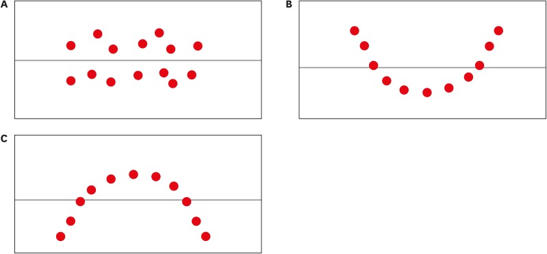
If the correlation coefficient is zero, there is also some caution needed in interpreting the meaning. We may expect no relationship such as Figure 3A, the shape of random scatter. However, U shape or reverse U shape relationship can show zero correlation coefficient (Figure 3B and 3C). An example of U shape relationship is the relationship between consumption of electricity and temperature. At very low temperature lots of electricity is consumed for warming and the need is gradually decreased with the increase of temperature. However, if temperature rises further we need more electricity for air conditioning. An example of reverse U shape is the relationship between stress and work performance. Performance may be improved if there is some stress, but too much stress can cause burn-out of the person which decreases performance. Therefore, it is always a good idea to examine the relationship between variables with a scatterplot.
SPEARMAN'S RANK CORRELATION COEFFICIENT
Spearman's rank correlation coefficient is the non-parametric version of the Pearson correlation coefficient calculated using rank values of two variables. It is expressed as following formula.

where d = Rank(Y) − Rank(X) and n = sample size.
While the Pearson correlation assesses linear relationships, Spearman correlation assesses monotonic relationship that two variables are related but not necessarily linear. Let’s consider the relationship between 99 p values ranges from 0.01 to 0.99 by 0.01-unit increase and corresponding log odds values,  . As seen Figure 4, Spearman correlation coefficient is 1 when y values always increase as x values increase, while Pearson correlation coefficient counts only linearity with coefficient of 0.97. Spearman rank correlation coefficient can be applied on continuous variables with influential outliers which are located far away from most observations. In such cases, it is not appropriate to apply Pearson. Also, it can be applied to assess relationships between ordered categorical values. The range of Spearman correlation coefficient is from −1 to +1, which represent perfect negative and positive relationships, respectively.
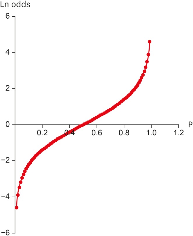
A curved relationship of ‘p’ and ‘ln odds’. (Pearson correlation = 0.97 vs. Spearman's rank correlation = 1).
Table 2 shows the calculation procedure of the Spearman rank correlation. Difference of rank of two variables is used in calculating rank correlation coefficient.
Appendices
Appendix 1
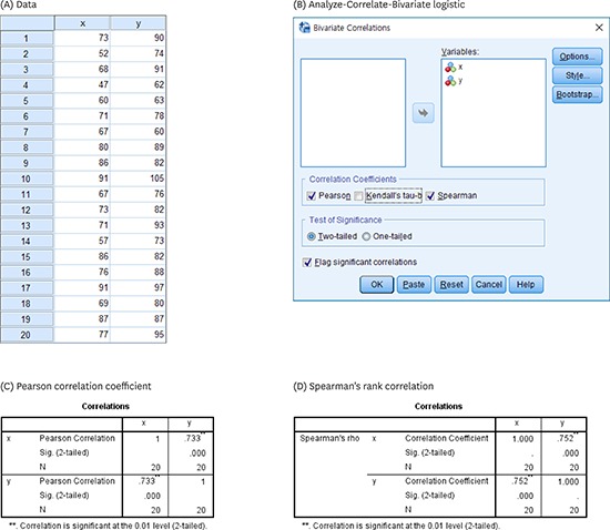
Procedure of covariance and correlation using IBM SPSS
The procedure of logistic regression using IBM SPSS Statistics for Windows Version 23.0 (IBM Corp., Armonk, NY, USA) is as follows.
